Deriving equations always have been a fascinating thing, due to current project requirement I recently started reading All of Statistics, in several chapters it omit some proofs which I'm going to outline here
The properties of conditional expectations.
First we lay down the definition of conditional expectations, if ![]() and
and ![]() are two random variables, then
are two random variables, then
![]()
where ![]() , as expected.
, as expected.
Notice that ![]() is itself a function of
is itself a function of ![]() , and
, and ![]() itself can be functions, just like in normal expectations, we have
itself can be functions, just like in normal expectations, we have
![]()
This is in fact a not so obvious result, because normally by definition of expectation we should have
![]()
The proof I will omitted here but it's nonetheless named Law of unconscious statistician. Today we simply want to discuss some of its properties, which are easy and fun to derive while remaining not-so-trivial.
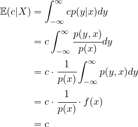
Theorem 1: ![]() , where
, where ![]() is a constant.
is a constant.
Proof:
(1) 
The author mentioned specifically about the regression problem, we use the function ![]() to represent the result of the regression, and if
to represent the result of the regression, and if ![]() is the random variable of the value on the de facto curve, then we can use the random variable
is the random variable of the value on the de facto curve, then we can use the random variable ![]() to represent the error between the result of regression and the real curve, the books says that if we let
to represent the error between the result of regression and the real curve, the books says that if we let ![]() , then
, then ![]() . To show this, we need first to establish a lemma.
. To show this, we need first to establish a lemma.
Lemma 1: ![]()
Proof:
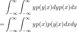
(2) 
Notice in the first step, since ![]() is a function
is a function ![]() of
of ![]() , thus when we expand the outer expectation we are actually expanding
, thus when we expand the outer expectation we are actually expanding ![]() for some
for some ![]() , thus we first integrating w.r.t.
, thus we first integrating w.r.t. ![]() , and when we expand further the inner expectation
, and when we expand further the inner expectation ![]() itself, by definition it's an expectation of
itself, by definition it's an expectation of ![]() so we are integrating w.r.t.
so we are integrating w.r.t. ![]() . Now, since
. Now, since ![]() itself is a constant w.r.t.
itself is a constant w.r.t. ![]() , we can move it inside the inner integral, and furthermore, in statistics we often make some aggressive assumptions, for example, here we suppose that the iterated integral automatically satisfies the Fubini's theorem, thus we can exchange their order,
, we can move it inside the inner integral, and furthermore, in statistics we often make some aggressive assumptions, for example, here we suppose that the iterated integral automatically satisfies the Fubini's theorem, thus we can exchange their order,
(3) 
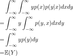
But notice that ![]() is just
is just ![]() ,and since
,and since ![]() is constant w.r.t.
is constant w.r.t. ![]() we can move it out of the inner integral, thus
we can move it out of the inner integral, thus
(4) 
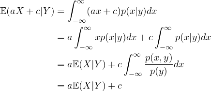
Having proven this, we need to prove another lemma, that is the linearity of conditional expectation, which the author also lacks in the original text
Lemma 2: ![]()
Proof:
(5) 
Now we can prove that ![]() by noticing that
by noticing that
(6) 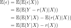
This means that the error between the result of regression and the actual curve can be modeled by a distribution whose expectation is ![]() , in fact, you should have no surprise that normally the error
, in fact, you should have no surprise that normally the error ![]() is modeled by a normal distribution centered at
is modeled by a normal distribution centered at ![]() , i.e.
, i.e. ![]() . That is, every curve regression problem can be modeled by the result of regression, plus a perturbation function
. That is, every curve regression problem can be modeled by the result of regression, plus a perturbation function ![]() that follows the normal distribution centered at
that follows the normal distribution centered at ![]() .
.


Comments NOTHING